Assessing the Empirical Validity of the Federal Reserve’s 2026 Global Market Shock Scenarios

Key Points:

• The Federal Reserve’s 2026 stress test proposals make GMS scenario development more transparent and accessible to public feedback.
• Empirical analysis demonstrates that the majority of GMS shocks surpass historical extremes and do not coincide, thereby raising concerns regarding their plausibility.
• The Federal Reserve may consider eliminating the GMS component or modifying the severity of GMS scenarios and the method of loss aggregation to account for diversification benefits across asset classes.

Background

On October 24, 2025, the Federal Reserve unveiled proposals to enhance the transparency and public accountability of its annual stress test. ¹ Key elements include: the Global Market Shock (“GMS”) scenarios for the 2026 test and the relevant GMS models.  This initiative grants the general public its first-ever opportunity to gain insight into the GMS development process and to provide formal feedback to the Federal Reserve.

What quantitative criteria does the Federal Reserve employ to define the severity of stress scenarios?

For firms engaged in significant capital market activities, the Federal Reserve employs the Trading Issuer Default Loss (IDL) model and the GMS to project potential losses.  These two components are calibrated according to separate quantitative criteria; however, the justification for employing divergent criteria remains unexplained.

The trading IDL model calculates potential jump-to-default losses across a nine-quarter horizon for individual firms and segments. The Federal Reserve then selects the 93^rd percentile of these loss distributions to represent a stressed scenario consistent with the severity of a major recession. The justification for selecting the 93^rd percentile is as follows:

“The 93rd percentile is chosen based on the frequency of severe recessions.  More specifically, in the sixty years from 1956 to 2015 (with 2015 corresponding to the year when this practice was first adopted), nine recessions occurred, four of which were severe.  Thus, the calculated frequency of severe recessions is four in sixty years or roughly an event that happens once every fifteen years.  This frequency suggests a draw from the 93rd percentile of the jump-to-default distribution.” ²

Whereas in determining the GMS scenarios, the Federal Reserve considers “Severe shocks fall within the historical minimum (including) and the 1st (less than) percentile or within the 99th (greater than) percentile and the historical maximum (including).” ³

The GMS models are calibrated to the 90^th percentile to simulate stressed yet plausible market scenarios.  It follows a stepwise approach: secondary risk factors are estimated based on primary ones like the S&P 500, with remaining factors modeled after both.  Most secondary risks use univariate quantile regression, which limits the model’s ability to capture historical correlations.  Consequently, the combined shocks may not adequately reflect historically observed relationships between risk factors.

Why are the Federal Reserve’s 2026 GMS scenarios not empirically plausible?

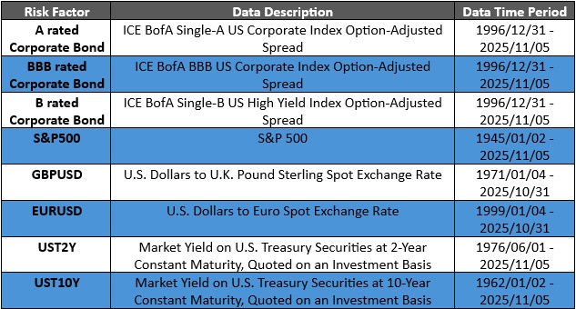
To assess the plausibility of the 2026 GMS scenarios, we identify eight key risk factors and present empirical percentiles alongside the dates of historically comparable shocks.  The Federal Reserve posits that severe market disturbances often occur concurrently during financial crises—an assertion substantiated when these shock dates are found to be closely aligned.

Currently, GMS scenarios feature over 20,000 risk factors, but the Federal Reserve proposes to reduce this to about 2,300 disclosed risk factors.  Our analysis focuses on eight: A Bond, BBB Bond, B Bond, S&P500, GBPUSD, EURUSD, UST2Y, and UST10Y (see Table A1 in the Appendix for details).

To develop the time series of historical shock values for each risk factor, we calculate these values using LH-day data windows, where LH represents the liquidity horizon for which the shock is calibrated.  The GMS models’ documentation specifies the liquidity horizon for each asset class. ⁴ These horizons are selected to align with the Fundamental Review of the Trading Book (FRTB), which defines liquidity horizons in terms of business days. ⁵ Accordingly, a one-month liquidity horizon is assumed to consist of 20 business days, consistent with FRTB standards.

Table 1 displays the empirical quantile for the 2026 GMS shock corresponding to each risk factor, along with the date of the most similar historical shock. The empirical quantile is determined from the historical distribution of shock values specific to each risk factor. Additionally, the table includes the 90^th percentile of each risk factor’s empirical distribution.

Table 1. 2026 GMS Scenario Quantile & Correlation Analysis.

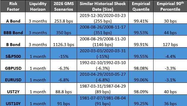
Table 1 shows that for single A rated corporate bonds in advanced economies, the 2026 GMS spread shock is 253.8 bps. The closest historical shock (255 bps) occurred from 2019-12-30 to 2020-03-23 during COVID-19. Table 2 uses this period as a reference to present empirical quantiles of shocks for the other seven risk factors within their respective liquidity horizons.

Table 2. Empirically coherent risk factors shocks, using the time frame of the historical shock to the single A rated bond spread (i.e., A Bond) most similar to the 2026 GMS scenario as the reference period.

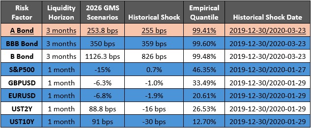
Two points are readily apparent:

1. The prescribed 2026 GMS shocks generally exceed the 99^th percentile of their historical range, surpassing the 93^rd percentile in the trading IDL model and the 90^th in the GMS models.
2. Comparable historical shocks are spread out over time, so severe events across asset classes do not coincide, highlighting diversification benefits.

Therefore, it is not empirically plausible to assume all extreme shocks occur together, as supported by the 2019 SIFMA GMS study. ⁶

What are the possible solutions?

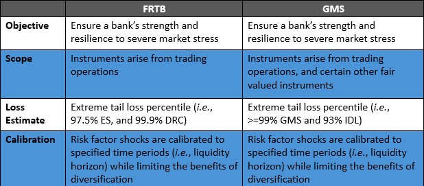
Our earlier blog posts have shown that the GMS component contributes to SCB volatility ⁷ and overlaps with market risk capital rules like the FRTB under Basel 3 Endgame. ⁸ The Federal Reserve might remove the GMS from supervisory stress tests, as it is not empirically plausible and overlaps with the FRTB.  Table 3 highlights conceptual similarities between the FRTB and the GMS.

Table 3. Conceptual similarities between the FRTB and the GMS.

 If the GMS component is retained, it’s recommended that the GMS scenarios adopt a more practical, empirical approach by choosing a lower percentile than what is used for the trading IDL model (i.e., the 93^rd percentile)—for example, using the 90^th percentile.  Such an approach would align with current market risk rules, ⁹ where VaR models use a lower percentile (99^th) than the Incremental Risk Charge model (99.9^th)—capturing issuer default losses as the trading IDL, and with the FRTB standards: 97.5% Expected Shortfall (“ES”) for general market risk losses (as in the GMS) and 99.9% Default Risk Charge (“DRC”) for issuer jump-to-default losses (as in the trading IDL).

Furthermore, to account for diversification benefits between asset classes, GMS loss estimates should be combined across different asset types using an FRTB-style aggregation method, similar to how delta risk capital is aggregated across risk factor buckets: ¹⁰

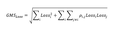
Here,  represents asset class  and  denotes supervisory-specified correlation between asset classes , .  The 2026 GMS Scenario Quantile & Correlation Analysis indicates that  should be near zero.

Conclusion

The Federal Reserve’s proposed 2026 Global Market Shock scenarios and GMS models aim to increase transparency in stress tests, but the scenarios are implausible, with shocks exceeding historical norms and lacking real-world clustering.  The Fed should consider removing the GMS component (because of its empirical implausibility and overlaps with the FRTB) or revising scenario severity and aggregation methods to account for diversification benefits across asset classes.

Appendix

Table A1. Description of GMS risk factors selected for the empirical quantile and correlation analysis. Data source: Federal Reserve Bank of St. Louis 

Author

Dr. Guowei Zhang is a Managing Director and Head of Capital Policy of SIFMA.

Footnotes